Create a P&L in Excel: A Practical Guide
If you are new to a finance and accounting role such as Financial Due Diligence (FDD), Transaction Services (TS), Investment Banking (M&A), Financial Planning & Analysis (FP&A), or Controlling, you will inevitably need to turn raw accounting data into a profit and loss statement (P&L) in Microsoft Excel at some point.
Having completed this task hundreds of times in my career, I will show you how to create a profit and loss statement in Excel efficiently. Together, we will:
Start with a trial-balance data export
Map / allocate detailed accounts to broader P&L categories
Build a P&L in Excel with both SUMIFS formulas and a PivotTable
You will learn not only how to build a P&L in Excel but also how to apply lookup formulas, aggregation techniques, mapping concepts, grouping methods, and other essential Excel skills used by top-performing finance professionals. Alongside the technical Excel work, you will get a feel why a strong grasp of accounting is equally important.
Preview: What You Will Create
By the end of this guide you will have two fully working versions of the same P&L:
A formula-driven P&L powered by SUMIFS, which is flexible and easy to format
A PivotTable P&L that you can collapse, expand, and use for fast analysis and quick iterations
Both approaches start from the same trial-balance extract, allowing you to cross-check the numbers easily.
These outputs provide a solid base to which you can add further KPIs and analytics such as margins, growth rates, and variances.
Formula-Driven P&L with SUMIFS
The profit-and-loss (income-statement) layout below uses SUMIFS to pull account values and then rolls them up with SUM or SUBTOTAL formulas.
This is the standard method among market leaders in mergers and acquisitions (M&A), transaction services (TS), and related finance and accounting disciplines.
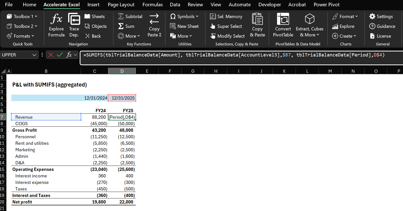
Exhibit 1. SUMIFS-driven P&L in Excel
PivotTable-Driven P&L
The alternative layout below is built with a PivotTable. You can collapse or expand periods, switch between yearly and quarterly views, show subtotals such as Gross Profit and Operating Expenses, or drill into granular lines like Personnel Expense.
This method is less common and tends to be favored by tech-savvy finance professionals. When set up correctly, a PivotTable P&L is extremely powerful, but it requires a bit more setup and Excel know-how than the straightforward SUMIFS approach.
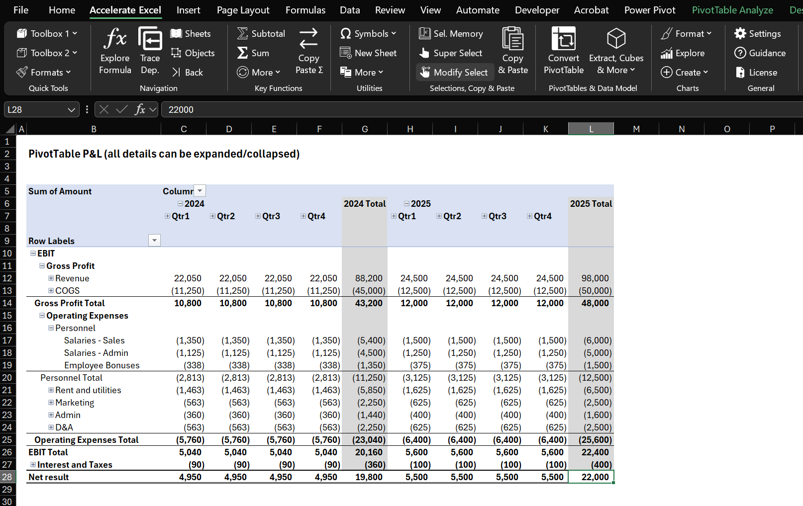
Exhibit 2. PivotTable-Driven P&L in Excel
Note: You might notice EBIT and Gross Profit appear at the top. PivotTables place group headers first by design. This behavior makes PivotTables excellent for quick analysis yet encourages many users to switch to formula-based spreadsheets for formal reporting. Our automatic conversion tool can turn a PivotTable into a formula-based report if you prefer that layout.
Want to build a balance sheet Pivot Table instead? Check out: Create a Balance Sheet PivotTable in Excel .
Starting Point: Trial-Balance Data
Most P&L-building exercises begin with an export from the accounting system, typically a trial-balance extract. A trial balance lists every account in the general ledger (GL) together with its ending balance after all entries and transactions have been posted.
A trial balance usually covers all account types—assets, liabilities, equity, income, and expenses. To create an income statement, we look only at income and expense accounts because those feed into the P&L.
Below is a simplified sample trial balance extract that contains only the P&L accounts used in this example.
To get the sample data, download the practice file.
| Account No. | Account Name | Period | Amount |
|---|---|---|---|
| 4000 | Product Sales - Online | 12/31/2025 | 60000 |
| 4001 | Product Sales - Retail | 12/31/2025 | 35000 |
| 4010 | Service Income | 12/31/2025 | 5000 |
| 4100 | Sales Returns - Online | 12/31/2025 | -1200 |
| 4101 | Sales Returns - Retail | 12/31/2025 | -800 |
| 5000 | Raw Materials - Plastic | 12/31/2025 | -15000 |
| 5001 | Raw Materials - Electronics | 12/31/2025 | -10000 |
| 5010 | Manufacturing Labor | 12/31/2025 | -18000 |
| 5020 | Packaging Materials | 12/31/2025 | -2000 |
| 5030 | Shipping Inbound | 12/31/2025 | -1500 |
Note: Some accounting exports present a single “Amount” or “Balance” column, while others split figures into separate debit and credit columns. Revenue and income usually appear as credit balances, which may be shown as negative numbers. If so, multiply those values by −1 so that income is positive and expenses are negative.
Keeping opposite signs for income and expenses is a small but critical practice. It lets you rely on plain addition in every step that follows, streamlining your work and reducing the risk of errors.
Data Preparation
Side Note on Mapping Tables: Account and Line-Item Hierarchy
Before diving into Excel formulas, understand the hierarchy-mapping concept. A hierarchy mapping table links each granular item (for example, a raw GL account) to an aggregated P&L category or line item.
In other words, you create a bridge between the detailed accounts in the trial balance and the higher-level sections you want to show on the P&L report.
Why build an account hierarchy mapping table?
Summarization. Assign each account to a category such as Revenue, Cost of Goods Sold, or Operating Expenses, and you can total those categories with simple formulas.
Consistency. Once the mapping exists, you can reuse it for future periods. If the trial balance later contains new numbers or new accounts, drop them in; the summary formulas keep working. Only truly new accounts need to be added to the mapping table.
Clarity. The exercise forces you to decide where each account belongs. This is invaluable in valuation or due-diligence work, where you may need to align a company’s chart of accounts with a standard layout.
Quick changes. Need a particular GL account to roll into a different P&L line item? Edit the mapping, and the summary updates automatically. There is no need to rewrite complex formulas; maintain the mapping table instead.
For the sample data above, a (shortenend) account-mapping table might look like this:
| Account No. | AccountLevel1 | AccountLevel2 | AccountLevel3 | Account Name |
|---|---|---|---|---|
| 4000 | EBIT | Gross Profit | Revenue | Product Sales - Online |
| 4001 | EBIT | Gross Profit | Revenue | Product Sales - Retail |
| 4010 | EBIT | Gross Profit | Revenue | Service Income |
| 5000 | EBIT | Gross Profit | COGS | Raw Materials - Plastic |
| 5001 | EBIT | Gross Profit | COGS | Raw Materials - Electronics |
| 5010 | EBIT | Gross Profit | COGS | Manufacturing Labor |
| 6000 | EBIT | Operating Expenses | Personnel | Salaries - Admin |
| 6001 | EBIT | Operating Expenses | Personnel | Salaries - Sales |
| 6100 | EBIT | Operating Expenses | Rent and utilities | Rent - Office |
| ➕ Click to Expand All | ||||
How to Map Accounts
Creating the Mapping Table
So, how do you create a mapping table? You have several options:
Create it manually on a separate worksheet or next to your trial-balance data.
Import an existing mapping from your accounting system.
Write a script to automate part of the process.
Experiment with AI to generate a first draft (my experience has been mixed, and I often find that manual work is faster).
Manual vs. Automated Mapping
If you cannot extract a mapping from your accounting system, building it by hand is usually the quickest approach. It is mostly a one-off exercise, and it forces you to review every general-ledger account, which is always worthwhile.
Even when you can automate part of the task, keep an option to do manual adjustments. The mapping table gives you fine-grained control over your final output and reporting structure.
Adding Mapping Information to the Data
After the mapping table is ready, integrate it with your trial-balance data by using lookup formulas such as:
XLOOKUP or VLOOKUP
Each formula searches for the account number in the mapping table and returns the corresponding category.
For simplicity, we will place everything in one large data table rather than multiple related tables (those are common in more advanced star-schema data models). More advanced techniques that use Power Query and Power Pivot (Excel’s Data Model) will appear in a separate article and will be cross-referenced here later.
Step-by-Step Guide to Prepare Data
Practice File and Sample Data
To get the most out of this tutorial, pick one of the following options download the practice Excel file. It contains the sample data, solutions, and several alternative starting points.
Introductionary Notes
Table references. We will store data in an Excel Table so that structured references such as
tblDataTrialBalance[Amount]can be used. They read more clearly, and Tables expand automatically as new rows are added. If you would rather work with standard ranges, be sure to size them generously so they still cover any future rows.Detailed shortcuts. I list keyboard shortcuts, which I usually use. Treat them as guidance, not mandatory steps.
Step 1: Convert Raw Data to a Table
On the RawData sheet, click any cell inside the data range and press Ctrl + A.
Press Ctrl + T → Enter.
Select the table and navigate to Table Design on the ribbon, then to Table Name: on the left and enter tblTBData.
Step 2: Prepare the Account Mapping
Copy the Account No. and Account Name columns
Press Ctrl + Home.
Hold Shift, press the Right Arrow, then hold Shift + Ctrl and press the Down Arrow.
Press Ctrl + C.
Move to cell K1:
Press Ctrl + Up Arrow to return to row 1.
Press Ctrl + Right Arrow to reach the right edge of the current data block.
Press Right Arrow repeatedly (or use mouse) until cell K1 is selected.
Paste into cell K1 with Alt → E → S → V → Enter.
Remove duplicates
Ensure the two pasted columns remain selected, or re-select them.
Press Alt → A → M → Tab → Tab → OK (or use Data → Remove Duplicates).
Add three new category columns
In cell M1 type AccountLevel1.
In N1 type AccountLevel2.
In O1 type AccountLevel3.
Populate the category columns
AccountLevel
Enter EBIT for accounts that belong to EBIT (Earnings before Interest and Taxes). In this example, EBIT includes all accounts except those starting with 7. Enter Interest and Taxes for the rest.
AccountLevel2
Enter Gross Profit, Operating Expenses, or Interest and Taxes.
Gross Profit: accounts starting with 4 or 5.
Operating Expenses: accounts starting with 6.
Interest and Taxes: accounts starting with 7.
AccountLevel3 (detailed categories)
Enter the detailed P&L line items.
Revenue: starting with 4
COGS: starting with 5
Personnel: starting with 60
Rent and utilities: starting with 61 and 62
Marketing: starting with 63 and 64
Admin: starting with 65 and 66
D&A: starting with 67
Interest income: starting with 70
Interest expense: starting with 71
Taxes: starting with 72
Note: In practice, a solid finance and accounting knowledge is essential for this step.
Step 3: Merge Account Mapping with Raw Data
Create INDEX / MATCH formula in cell E2
Type =INDEX(
Select column AccountLevel1 in the account mapping table
Type ,MATCH(
Click on cell B8
Type ,
Select column Account No. in the account mapping table
Tip: select any cell in that column and press Ctrl + Shift.
Type ,0)) and press Enter.
Optional: Press Alt + Enter to insert line breaks for better formula readability.
Repeat for AccountLevel2 and AccountLevel3
Copy-paste the formula two columns to the right for AccountLevel2 and AccountLevel3.
Adjust the column names in the table header.
Make sure your formulas reference the correct columns.
Now, we are done with the boring part and are all set to start creating some P&Ls!
Create P&L Using SUMIFS Formulas
The first, and most common, method to build a P&L is to use Excel’s SUMIFS function to aggregate trial-balance values by the categories we defined.
Aggregated vs. Detailed P&L
When you use SUMIFS, you must decide the level of aggregation.
Aggregated (high-level) P&L with SUMIFS
In this version each row represents a full category—for example, total Revenue and total Cost of Goods Sold (COGS). A single SUMIFS formula adds every account assigned to that category.

Exhibit 3. SUMIFS-driven P&L aggregated by top-level sections such as Revenue and COGS
Trial-balance-level (detailed) P&L with SUMIFS
In the detailed layout each row shows one trial-balance account, and SUM formulas roll those accounts up into their parent categories.
Grouping and indentation allow you to collapse or expand detail, so the worksheet stays polished and readable even when it contains many lines.
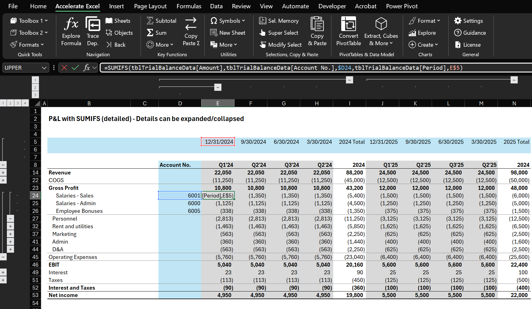
Exhibit 4. SUMIFS-driven P&L calculated bottom-up at the trial-balance-account level
SUMIFS Basics
The SUMIFS formula sums a range based on one or more criteria. Here we will sum the Amount column, provided that:
The row in AccountLevel2 matches the category in B5.
The row in Period matches the date in D3.
=SUMIFS(tblTBdataMapped[Amount], tblTBdataMapped[AccountLevel2], $B5, tblTBdataMapped[Period], D$3)
If you are new to SUMIFS, read our article on this topic.
When to Use SUMIFS
You will almost always create a SUMIFS‑driven P&L for reporting and analysis. SUMIFS formulas are dynamic and let you customise structure, format, and layout.
The real question is which level of granularity you need. Aggregated P&Ls are quick to set up and make an excellent sanity check for other methods. Detailed P&Ls may offer more insights but can be time‑consuming to maintain, so weigh the effort against the insights gained. Consider:
Will you gain additional insights, or spend hours for minimal value?
Who is the recipient, and what is the context?
Is this a one‑off or recurring task?
How stable is the chart of accounts?
How much time do you have?
A practical approach is to maintain:
A moderately aggregated P&L for quick insight, summaries and low maintenance.
A bottom‑up PivotTable P&L with all the granular details, giving you the ability to perform drill-downs on short notice.
| Category | Aggregated P&L (SUMIFS) | Detailed P&L (SUMIFS) |
|---|---|---|
| Advantages |
• Super-fast to spin up • High-level view is less noisy when new GL accounts pop up |
• Full transparency – every GL line shows • Easier to trace odd movements without drilling into another sheet |
| Disadvantages | • No line-item context, so root-cause hunting can be a pain |
• Heavier workbook (lots of rows & formulas) • More fragile – add one rogue account or typo and the whole thing can break • Slower to calculate on big data sets |
| When to Use | Pretty much always as a “front page” snapshot for management packs |
• Preparing work to be shared externally (e.g. financial models, M&A/financial due diligence datapacks) • One-off / adhoc work • When you have a stable charter of accounts |
How to Create P&L with SUMIFS (Step-by-Step)
Starting Point
We begin with the trial-balance data merged with the accounting mapping in the Excel table named tblTBData.
If you have not built tblTBData yet, you have two options:
Build it yourself by following the steps in the Data Preparation section.
Skip ahead to the SUMIFS section and use the pre-transformed and formatted source data in the practice workbook (table tblTBDataSolution on the Solution_Source_TBdata sheet).
Step 1: Prepare the P&L Construct
Create a new sheet for the P&L and copy the account hierarchy
Create a new worksheet.
Go to Solution_Source_TBdata. Confirm that columns AccountLevel1 → AccountLevel3 are in the right order.
Click any cell with a value in the AccountLevel1 column, then Ctrl + Space → Space to select that column including header.
Add column AccountLevel2 and AccountLevel3 to the selection by holding Shift and pressing Right Arrow twice.
Press Ctrl + C.
Switch to the new sheet (Ctrl + Page Down).
Select cell C9 and paste with Alt → E → S → V → Enter (values-only).
Remove duplicates from the pasted hierarchy
Select the range you just pasted.
Run Data → Remove Duplicates or press Alt → A → M → Tab → Tab → Enter.
Prepare the period labels
Go to Solution_Source_TBdata and copy the Period column.
Paste it onto the new sheet in cell G12, remove duplicates, then sort ascending (Data → Sort → Ascending or Alt → A → S A).
Copy that clean list, go to cell G9, and paste transposed with Alt → E → V → E → Enter.
Delete the original column you pasted by clearing contents and formats with Alt → H → E → A.
Step 2: Build SUMIFS formula
=SUMIFS(tblTBdata[Amount], tblTBdata[AccountLevel3], $B8, tblTBdata[Period], F$7, )
Create SUMIFS formula in cell G11
Type =SUMIFS(
Select column Amount in Table tblTBDataSolution
Type ,
Select column AccountLevel3 in Table tblTBDataSolution
Type ,
Go back to your worksheet and click on cell E10 (or type it). Press F4 three times to anchor the column reference. Make sure you remove the reference to your worksheet (i.e. it should read $E10 and not Sheet1!$E10). Here is why.
Type ,
Select column Period in Table tblTBDataSolution
Type ,
Click on cell F9 (or type it). Press F4 twice to anchor the row reference.
Press Enter.
Copy the formula
Select the cell with your SUMIFS formula and press Ctrl + C.
Select the range to paste the SUMIFS (G10:G20). Paste formulas with Alt → E → S → F → Enter.
Step 3: Finalize the P&L
Add subtotal rows
Insert a blank row after each AccountLevel2 group (for example, below the Gross Profit block).
Navigate to the first cell with the next group and press Ctrl + Shift → + . This will insert a row and shift the remaining cells down.
Copy and paste the name of the group into the AccountLevel3 column.
Repeat for all groups.
Insert a blank row after Operating Expenses and name it EBIT.
In the value columns, enter a SUM (or SUBTOTAL) that totals the rows above.
In cell G12, enter: =SUM(G10:G11)
In cell G18, enter: =SUM(G13:G17)
In cell G23, enter: =SUM(G19:G21)
Add a grand total row
Insert a final row labeled Net Income.
In cell G24, enter: =SUM(G12,G18,G23).
Apply final formatting
Format each subtotal row and the grandtotal row in bold.
Add borders to separate major sections.
Select the header row and navigate to Home → Borders → Thick Bottom Border.
Select the subtotal rows and navigate to Home → Borders → Top Border.
Select the grand total row and navigate to Home → Borders → Top and Double Bottom Border.
Use an appropriate number format with suitable decimals.
For example, select the values cells (G10:G23), right-click and navigate to Format Cells → Number Format → Custom → Enter:
#,##0_);(#,##0);" - "_);@_) and click OK.
Note: For this to work properly you must use the same locale as me (US).
Further fine-tuning as needed. From here, you can do some more formatting, add KPIs, variance columns, add checks to the source data, and so on.
Create P&L Using Pivot Table
Recap: PivotTable Basics
Pivot Tables summarize data quickly in Excel. They can turn a trial balance into a P&L with a few clicks. Pivot Tables handle grouping and summation without worksheet formulas.

Exhibit 5. Example of a PivotTable-driven P&L in Excel (bottom-up calculated at trial-balance account level)
When to Use Pivot Tables
Pivot Tables are great when you do not yet know what you are looking at:
You can slice and dice, change views and play around with data quickly
You get answers about total revenue or expenses as well as detailed drill-downs on financial statement line items and trial balance accounts.
For presentation or modeling, formula-based P&Ls give you tighter layout control. Use both approaches: keep a PivotTable for validation and deep dives, then build a formula version for the final output. Having the PivotTable in reserve makes it easy to handle ad-hoc questions.
However, keep in mind that a strong PivotTable P&L depends on well-structured source data, so weigh the setup effort against the project scope:
Short, ad-hoc work (a few days). Skip the PivotTable unless you receive clean, structured data and can set it up in minutes.
Longer projects (multi-month sell-side mandates or in-house finance work). The upfront investment usually pays off.
| Pivot Table Pros | Pivot Table Cons |
|---|---|
| Speed: Create a pivot summary in seconds. Perfect for quick analysis of large trial balances. | Limited formatting flexibility: Pivot tables have preset layouts. They do not offer the same level of customization as standard worksheet cells. |
| No formulas required: Built-in summarization reduces formula errors. | Need to refresh: Unlike formulas, pivot tables need manual refreshing after data changes. |
| Automatic inclusion of new accounts: Refresh the pivot to include newly added accounts. No need for new SUMIFS formulas. | Learning curve: New users may need time to learn the interface. |
| Drill-down capability: Double-click any number to see underlying transactions or accounts. | Data structure requirements: Your data must be well structured for pivots to work properly. |
| Quick comparisons: Create side-by-side P&Ls for multiple periods if your data includes them. |
How to Build a P&L Pivot Table (Step-by-Step)
Starting Point
We begin with the trial-balance data merged with the accounting mapping in the Excel table named tblTBData.
If you have not built tblTBData yet, you have two options:
Build it yourself by following the steps in the Data Preparation section.
Skip ahead to the PivotTable section and use the pre-formatted data already in the practice workbook (table tblTBDataSolution on the Solution_Source_TBdata sheet).
Step 1: Insert the PivotTable
Create a new sheet and select cell C6.
Go to ribbon Insert → PivotTable → From Table/Range.
Switch to worksheet Solution_Source_TBdata, click any cell in the data table, and press Ctrl + A to highlight the entire table.
Click OK to create the PivotTable on the new sheet.
Step 2: Populate the PivotTable
Navigate to the PivotTable Fields pane.
Drag AccountLevel1, AccountLevel2, AccountLevel3, and AccountName to Rows.
Drag Period to Columns.
Drag Amount to Values.
Step 3: Adjust Layout & Format
Click anywhere inside the PivotTable.
Navigate to ribbon tab Design → Subtotals → Show All Subtotals at Bottom of Group.
Design → Grand Totals → On for Columns Only.
In the Pivot body, right-click any second-level item (for example COGS) and select Expand/Collapse → Collapse Entire Field.
Drag items to follow the natural P&L order—for instance, move Revenue above COGS.
Step 4: Fine-Tune the PivotTable
Right-click the PivotTable → PivotTable Options.
Clear Autofit column widths on update.
Check For empty cells show: and type 0.
In the Fields pane, right-click Sum of Amount → Value Field Settings → Number Format → Custom and apply your preferred format (for example:
#,##0_);(#,##0);"-"_);@_)Select the period headers, then Home → Alignment → Align Right to right-align them.
Your PivotTable now functions as a dynamic, drill-down P&L ready for analysis.
PivotTable Tips I Wish I'd Known Sooner
Without going into too much detail, let me name a couple of topics you should have heard about when using PivotTable.
Compact vs Tabular Layout: We used compact in this article as it is the closest to the standard SUMIFS P&L approach. However, you’ll also often see and use tabular layout, which lays out the mapping information into additional columns.
Repeat Items: If you opt for tabular layout, you often want to tick “repeat items” so that the additional columns actually resemble the mapping.
Show missing values as 0: Empty cells do not look great, which is way you can tell the PivotTable to show 0 instead (right-click the pivot → PivotTable Options).
Expand/collapse multiple hierarchies at once: For instance, right-click on an item of the hierarchy level you want to expand → Expand/Collapse → Expand Entire Field.
You can adjust styles to customize the format of the Pivot Table, for example to add subtotal borders: Select PivotTable → Design → PivotTable Styles → Modify.
You can sort by a column (note that unfortunatly there is no absolute sort option available, so if you want to sort expenses (negative) by magnitude, your revenue accounts (positive) will be in the wrong order).
You can find all the essential PivotTable tips and tricks here: Excel Pivot Tables: Tips for Finance Professionals
Some General Tips
Adopting sound practices spares you future headaches, below are two important aspects that you should keep and eye on.
Accounting Data and Account-Mapping Exports
Before you dive into analysis, review the data extracts available from your accounting system:
Understand your export options. Most systems can output data in several formats.
Avoid “report-style” exports that look good to the eye but are hard to work with in Excel; they often require heavy re-formatting, especially when building a PivotTable P&L.
Request or generate a raw, table-structured export (one row per transaction or trial-balance line, with separate columns for account IDs, amounts, periods, etc.). With well-structured data, the procedures in this guide take only minutes. With poorly structured exports, they can consume hours—or even days—of clean-up time.
Consistent Signs for Revenue and Costs
General rule – Keep all income figures positive and all cost figures negative. Building your entire P&L around additions instead of subtractions avoids sign errors and speeds up model-building.
How to enforce correct signs if data comes with a single sign:
Add a Sign column to your account-mapping table:
+1 for revenue and asset accounts.
-1 for expense and liability accounts.
Join the Sign column to the transaction table on AccountID, then multiply the transaction amount by Sign to set the proper sign automatically.
When stakeholders insist on positive costs. Maintain two versions:
A technical P&L that keeps true (negative) cost signs.
A presentation sheet that references the technical P&L but multiplies costs by -1 so they display as positive.
Monthly versus Year-to-Date (YTD) Data
Pull monthly values whenever possible and aggregate them to YTD yourself.
Working in the opposite direction—deriving monthly numbers from YTD totals—is time-consuming, error-prone, and restricts later analysis.
Be More Productive with Accelerate Excel
After spending considerable time crunching financial, accounting and sales data in Excel, I noticed certain tasks could run far more smoothly with a few extra tools. Together with like-minded colleagues, I developed Accelerate Excel, a productivity toolbar designed to make exactly the kind of work described in this article more efficient.
Here are several features that tie directly into building a P&L in Excel.
Convert PivotTable to Normal Cells
This function converts a PivotTable into regular cells—using either hard-coded values, SUMIFS, GETPIVOTDATA or even the more advanced cube formulas. The advantage is clear: once you have a ready-made PivotTable P&L, you can transform it into standard Excel cells instantly. For instance, you can flip the PivotTable from the “PivotTable” section into the P&L found in the “SUMIFS” section in seconds.
Insert SUBTOTAL Shortcut
Many power users prefer SUBTOTAL over SUM for totals. Although Excel provides a built-in shortcut for SUM, no equivalent exists for SUBTOTAL. Our add-in fills that gap with a quick-access SUBTOTAL shortcut.
Copy-Paste SUM/SUBTOTAL Only
Sometimes you need to copy only the SUM formulas (or SUBTOTAL formulas) from one column to another. Numerous factors can prevent you from simpy copying an entire column’s formulas—say, links to different source sheets for actuals versus budgets because you haven’t had time to build a pristine single source of truth.
Fill Down
Working with mapping data often requires multiple fill-downs (or fill left/right) at once. Excel’s native Fill behavior rarely suits these scenarios, prompting many users to craft elaborate formulas or perform fills manually. Our add-in includes an AutoFill tool tailored to our requirements, saving even more time.
Convert INDEX/MATCH or SUMIFS to a Direct (Static) Cell Link
While SUMIFS and INDEX/MATCH are generally perfectly adequate, there are moments—especially when sharing a model—when simplifying with direct cell links helps others grasp the file faster. This tool converts those formulas into straightforward links on demand.
Customizable Formatting Hotkeys
Shortcuts for frequently used formats (header rows, subtotal rows, total rows, etc.) let you work faster than Excel’s native options. Competing add-ins often “overdo” formatting—for example, applying colors but also changing font sizes, which you then must undo. Our tools let you retain full control over what each hotkey applies.
Grouping and Indentation Helpers
Consistent grouping and indentation keep workbooks tidy and readable. Our toolkit offers capabilities to:
Automatically apply grouping and indentation based on the hierarchy implied by
SUMformulas.Apply grouping according to existing indentation, for example, assigning grouping level 2 to all cells with one level of indentation.
Apply indentation based on row groupings, for example, indenting selected cells according to their row-grouping level.
With Accelerate Excel, you can leave the office earlier—or turn that extra time into work that gets you promoted faster.
Conclusion
Building a P&L in Excel from trial-balance data can feel a bit tricky at first, but the approach outlined here lets you do it quickly and effectively.
Let’s recap the key steps:
Start with the Trial Balance: Make sure the format aligns with your requirements and adjust it if necessary. Verify sign consistency.
Account Mapping: Create a simple mapping of accounts to the P&L lines you need.
Choose Your Excel Tools: Use SUMIFS for a custom layout, PivotTables for rapid analysis, or both.
Focus on Results First: Get a working P&L fast, polish formatting later.
By following this guide, a beginner in a finance role can take raw trial balance data and convert it into a clear P&L. As you gain experience you will refine the workflow – perhaps automating imports with Power Query or maintaining a template where you paste a new trial balance and everything updates – but the fundamentals stay the same: import, map, aggregate.