Excel Power Query: Combine Multiple Files

/ Blog / Excel Power Query: Combine Multiple Excel Files (2025 Guide)

If you regularly merge data from several Excel workbooks – for example, monthly sales reports or trial balance spreadsheets – you know how time-consuming it can be. Manually copying and pasting data from each file is tedious and prone to errors.

Microsoft Power Query (also known as Get & Transform Data) allows you to import and consolidate data from multiple Excel files in a repeatable, automated way.

In this tutorial, we will provide a step-by-step Power Query tutorial on combining data from several files into one. You will learn how to set up Power Query to gather all those monthly files into a single table with just a few clicks. This process is a game-changer for Excel automation and can simplify real business workflows by removing routine data preparation tasks.

1. What is Power Query?
2. Why Use Power Query for Data Consolidation?
3. Preparing Your Data Source (Files and Folder Setup)
4. Step-by-Step: How to Combine Multiple Excel Files in Power Query
5. The Power Query “Load To” Interface
6. Power Query in Action: Refresh for New Data
7. Conclusion
8. Next Steps
9. Frequently Asked Questions (FAQ)

What is Power Query?

Power Query is a built-in Excel feature for data connection, transformation, and automation. Power Query can connect to many data sources, including Excel, CSV, and databases (SQL servers, Azure, etc.). It can transform or clean the data, then load it into Excel. In Excel 2016 and later, Power Query is found on the Data tab under Get & Transform Data. In Excel 2010 and 2013, it is a free add-in.

The key benefit is that once you define a query (a series of data import and transform steps), you can refresh it at any time to pull updated data. This allows you to avoid repeating the same steps manually.

For combining multiple files, Power Query can merge several files with the same schema into one unified table. For example, if you have a folder of monthly files (such as department budgets or regional sales), Power Query can consolidate these files into a single view. Once set up, you only need to add the next month’s file to the folder. A simple Refresh in Excel will include the new data automatically.

Power Query is available on the Data tab under **Get & Transform Data**

Why Use Power Query for Data Consolidation?

Before we discuss how, let us consider why Power Query is the ideal tool to consolidate Excel files. Many advanced Excel users rely on manual methods or VBA macros to merge data. However, Power Query provides a more robust, repeatable ETL solution that is accessible to beginners and advanced Excel users, without coding.

Below is a comparison of manual versus automated data consolidation:

Aspect	Manual Consolidation (Copy-Paste or Formulas)	Power Query Consolidation (Automated)
Process	Manually open each file and copy-paste data into a master workbook, or use complex formulas.	Define a query once to import all files. No need to manually open or copy.
Effort & Time	Time-consuming, especially with many files. Repeat the process each month.	Initial setup takes a few minutes. Future updates require one Refresh.
Risk of Errors	High risk of human errors (missing a file, misaligning data, copy-paste mistakes).	Minimizes human error by using a consistent process every time.
Data Consistency	Formatting or column mismatches can be fixed manually each time.	Needs a consistent schema. Inconsistent data can be cleaned with steps.
Handling New Data	Adding a new monthly file requires doing all steps or editing formulas/macros again.	Adding a file to the folder is automatically detected. Refresh updates data.
Skills Needed	No special skills, but tedious for large tasks.	Point-and-click with Power Query. No code needed. Scales to large volumes.

Power Query streamlines an otherwise labor-intensive process. It reduces maintenance and the chance of mistakes.

Another big advantage is reproducibility. Once you create the query, you or anyone else can use it again next period with no extra steps. This is crucial in business workflows that require monthly or weekly reporting.

Finally, Power Query keeps an audit trail of each transformation step. You can see how the data was combined and cleaned, which helps troubleshooting and transparency. In short, Power Query frees your time for analysis and decision-making.

Preparing Your Data Source (Files and Folder Setup)

Before you begin in Excel, take time to prepare your files. Good setup helps ensure smooth consolidation.

Collect all source files in one folder
Create a folder for the Excel files you want to consolidate. Power Query will fetch every file in that folder. Do not mix in files you do not want included.
Ensure consistent column structure
Each Excel file should have the same columns with matching headings and data types. If a file has extra columns or fewer columns, Power Query might add columns as null or ignore them. Try to keep a standard layout across all files.
Use Excel tables or clean ranges
If possible, format each file’s data as an Excel Table. If not, make sure each worksheet’s data begins at cell A1 with a header row and no extra text or totals under the data.
File naming consistency (optional)
You do not need all files to have the same name, but a consistent pattern (for example, Sales_Jan.xlsx, Sales_Feb.xlsx) can help. Power Query can capture file names as a source identifier if you want to track which row came from which file.

With that done, you can now combine multiple Excel files in Power Query.

Step-by-Step: How to Combine Multiple Excel Files in Power Query

Open a new Excel workbook
This can be a fresh workbook or an existing one where you want the combined data.
Use Power Query to import from the folder
Go to Data. Click Get Data > From File > From Folder. This instructs Excel to import data from all files in that folder.
Select the folder that holds your source files
The preview window should show the files it finds. Make sure the files you want are there. If there are files you do not want, you can filter them later.
Combine the files
In the preview dialog, choose Combine & Load or Combine & Transform. Power Query uses the first file as a sample to detect structure. For Excel workbooks, pick the correct sheet or table (for example, Sheet1, Table1) that exists in all files.
Wait for Power Query to append the data
Power Query processes and stacks the data. You may see a column with the source filename. This helps identify which file contributed each row.
Check the merged data
Look at the new worksheet where Power Query placed the combined data. If something is not correct, select Transform Data to open the Editor. You can then remove unwanted columns or rows, rename headers, or change data types. Click Close & Load when done.
Save the workbook
This saves the query definition. Next time, you can refresh without redoing your steps.

You have successfully combined multiple Excel files with Power Query. You now have a single table containing all rows from your source files.

The Power Query “Load To” Interface

When you finish in the Power Query Editor, go to Home > Close & Load > Close & Load To.... This opens the Import Data dialog. It has three sections:

How to view the data: Table, PivotTable, PivotChart, or Only Create Connection
Where to put the data: A new worksheet or an existing worksheet
Add to the Data Model: A checkbox that also loads the data into the Excel Data Model (Power Pivot)

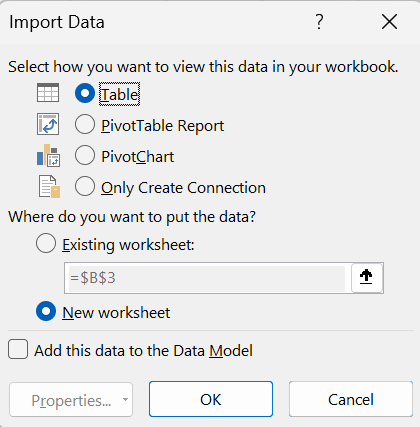
The Import Data (Load To) dialog in Excel Power Query

Option 1: Table

What it is: This is the standard output. The query results will be loaded as an Excel Table. (Note that this is also the default option and the output of step 7 above)

What it does technically: Excel creates a structured Table in a worksheet and fills it with the query result. The query is linked to that table, so any refresh overwrites the table’s contents with up-to-date data. You can identify a Power Query table by selecting a cell and seeing the Query contextual ribbon. The Queries & Connections pane will show “[X] rows loaded” next to the query name, indicating it is loaded to a worksheet table.

Because the data exists in the grid, note that Excel’s sheet limits apply. You cannot output more than 1,048,576 rows or 16,384 columns. If your query returns more rows, Excel will truncate or error out. Power Query can handle more rows in memory, but the sheet cannot display them.

When to use:

Good for visible, detailed data in Excel.
For data inspection or cleaning: you can scroll through actual rows, copy/paste, or do spot checks.
For using Excel formulas or charts on the data: since it is in cells, you can perform further analysis with SUMIFS, VLOOKUP, XLOOKUP, INDEX/MATCH or other standard formulas.
Suitable for smaller to medium datasets. Tables are fine for thousands or hundreds of thousands of rows if your system can handle it. Very large datasets will bloat the workbook and be slower. If you are near Excel’s row limits or the file becomes huge, consider using the Data Model instead.
Staging for external links: other workbooks or tools may read from a sheet. Loading to a table allows outside references.

Remember that an Excel Table output stores the data twice: once in Power Query’s internal cache while refreshing, and once in the worksheet itself. If you do not actually need each row in Excel, you might choose a PivotTable or Data Model for more efficiency. But for many everyday needs, a Table is perfectly fine.

Option 2 & 3: PivotTable or PivotChart

In my opinion you do not really need those as you can create PivotTables or PivotCharts separately, so feel free to skip. However, here is some detail.

What it is: This option loads the query result into a PivotTable or PivotChart. You will not see all rows in a table on the sheet. Instead, you jump to summarizing via the Pivot interface. After choosing PivotTable Report, Excel prompts for a location (new worksheet by default) and creates a blank PivotTable that links to the query’s data.

What it does technically: There are two ways Excel can store data for a pivot from Power Query:

If Add to Data Model is unchecked: the query output goes into an internal Pivot Cache (in-memory store for PivotTables). This is similar to creating a pivot from an Excel table. The pivot cache can inflate file size for large data.
If Add to Data Model is checked: the query output goes into the Data Model (Power Pivot). There is no traditional pivot cache. The pivot pulls data from the Data Model’s compressed storage. This is more memory-efficient and enables advanced features like DAX measures.

Either way, a PivotTable load does not create a visible worksheet listing of all data. You see only the PivotTable Fields list. You can drag columns into Rows, Columns, or Values to summarize.

Option 4: Only Create Connection

What it is: This tells Excel not to load the query results to any worksheet or PivotTable. The query is saved as a connection in the workbook’s Queries & Connections pane. No worksheet range is filled.

What it does technically: When you choose connection-only, Excel stores the query definition and credentials. On refresh, it caches the data internally, but does not display it on any sheet. You can still use it in other queries or load it to the Data Model. The Queries & Connections pane shows “Connection only.”

When to use it:

Staging or intermediate queries: if you plan to merge or append this query with others, you can keep it as a connection to avoid clutter on the worksheet.
Feeding the Data Model or Pivot: you can load the query to the Data Model by checking Add to Data Model. Then you build a pivot from the model. This avoids storing a duplicate pivot cache.
Large datasets exceeding Excel’s row limits: a connection-only query can handle millions of rows if they are not loaded to a sheet. You can then filter or aggregate that data in another query.
Behavior on refresh: connection-only queries update in memory on refresh, but you will not see them in the sheet. Dependent pivots or other queries can use this updated data.

Option 5: Add this data to the Data Model

This is not a standalone output but rather a supplemental option (a checkbox in the Load dialog) that can be used with any of the above choices.

What it is: The Data Model in Excel (also known as Power Pivot) is an in-memory relational data engine that Excel 365 uses to allow analysis across multiple tables and to efficiently store large datasets. (In essence, you are loading the data into the xVelocity (VertiPaq) engine – the same technology that powers Power BI’s datasets.)

What it does technically: If selected, after the query runs, Excel creates a Data Model table with the query’s data. You can view this by going to Data > Data Model in Excel. The table will appear there with the query name. The data in the model is highly compressed (columnar storage with encoding), often drastically reducing memory footprint compared to raw tables or pivot caches. The Data Model allows you to create relationships between tables and to create DAX measures for advanced calculations.

Important points on usage:

You can use Add to Data Model with Only Create Connection. This effectively loads the data only to the model without any visible sheet output. This is a common practice for building Power Pivot data models. For instance, if you import several tables (Customers, Products, Sales) and only add them to the Data Model, you can then define relationships and create PivotTables from the model.
You can use it with Table. In that case, the data will exist in two places: the worksheet table and the Data Model. This can be useful if you want a table for immediate use, but also want to combine that table with others in the model. Be aware it doubles storage. Excel is not smart enough to avoid duplication. It will load the same rows twice.
You can use it with PivotTable or PivotChart. If you check Add this data to the Data Model, the pivot will use the Data Model as its source. This is beneficial for performance with large data and for enabling features like distinct count or multiple data tables. If you forget to check it for a pivot and later realize you needed the model, you must change the query load or use Power Pivot’s “Add to Data Model” on the table, then recreate the pivot from the model.

When to use it:

Large datasets: The Data Model can handle millions of rows (limited by system memory) because of compression. It also bypasses the worksheet row limit.
Multiple tables / Relational Data: If your analysis involves more than one table (for example, sales and customers or trial balances and accounts), the Data Model is essential. It is the only way to create relationships within Excel and do multi-table pivots. In Power Query, you might output each relevant query as Connection Only + Add to Data Model. Then in Power Pivot’s Diagram View, you relate the tables (Sales table’s CustomerID to Customers table’s CustomerID). Your PivotTables (from the Data Model) can pull fields from both tables. This is exactly how Power BI’s data model works, and Excel’s is no different.
Advanced analytics and DAX: When data is in the Data Model, you can create calculated measures using DAX (Data Analysis Expressions), such as year-to-date totals, rolling averages, or distinct counts of customers. A regular pivot on a sheet-only cache cannot do these easily.
Reducing file size and improving refresh speed: Storing data in the Data Model often reduces file size significantly for large datasets. It can also make refreshes more efficient for pivots. If multiple pivots use the same Data Model table, they share one compressed copy of data, rather than each pivot having its own cache. Note that initially loading data to the model might be a bit slower than loading to a sheet, due to compression. The trade-off is usually worth it once you reach a certain data size.

In summary, Add to Data Model aligns Excel’s Power Query with modern BI workflows – it essentially treats Excel as a mini Power BI. By using the Data Model in Excel, you are using it the way Power BI would, which can be a good future-proofing if you plan to migrate or integrate with Power BI.

Power Query in Action: Refresh for New Data

One of the most powerful features of this setup is what happens when your data updates. Imagine it is next month and you receive a new Excel file to add to this consolidation. Normally, you would copy and paste the new data. With the Power Query solution, you only drop the new file into the same folder. Then you open your consolidated workbook in Excel and click Refresh All on the Data tab (or right-click the table and choose Refresh). Power Query will reconnect to the folder, find the new file, import its data, and append it to the table. Within seconds, your consolidated table updates to include the new entries. There is no need to redo any import steps – the query remembers the process.

Similarly, if a source file’s data changes (for example, a correction), a Refresh will pull in the updated values. This makes maintaining your reports very efficient. You can confidently say that your consolidated report always reflects the latest data with a single click. Power Query automation turns a repetitive task into a reliable refresh process.

Conclusion

Power Query allows you to import and consolidate many Excel workbooks into a single data source with ease. This automation reduces errors and saves hours of work. You can refresh your consolidated data any time, without repeating manual steps.

Power Query also offers a variety of data transformations, such as merging tables or cleaning column headers. These transformations can help you prepare more complex data for analysis. By mastering Power Query, you will be ready to tackle larger business problems in Excel with greater efficiency.

Power Query is built into Excel and offers a user-friendly interface, making Excel automation accessible even to those without programming skills. It is one of the best tools for intermediate and advanced Excel users who handle recurring data tasks. By investing time in creating a query, you gain the benefits of one-click updates and reliable data consolidation.

Once you automate your data consolidation with Power Query, you might wonder what other manual Excel tasks you can streamline. This is where the Accelerate Excel add-in can complement your workflow. Accelerate Excel is a productivity add-in that provides many one-click tools to speed up common Excel tasks. These tasks include advanced formatting, formula auditing, and managing worksheets. It is a great companion to Power Query. While Power Query automates data import and transformation, Accelerate Excel automates many in-workbook tasks that still take up time. Consider trying the add-in to further boost your productivity (you can download it and start a free trial here).

Next Steps

Explore the Excel Data Model (Power Pivot)
Once you have created a Power Query workflow, learning the Excel Data Model is often the next step. In fact, it is only one checkbox away. If you need advanced analytics or want to store large datasets, consider using the Excel Data Model. You can build relationships between tables and create powerful measures using DAX. Power Pivot works well with Power Query for a complete data solution.
Learn About Cube Formulas
Cube Formulas let you extract data from the Excel Data Model without building a large PivotTable. They allow you to control layout while still referencing values stored in the Data Model. This is useful if you prefer to write formulas in cells but want the advantages of Power Pivot (including filters and/or slicers).
Read this: Excel CUBE Formulas: A Must-Know for Data-Heavy Consulting Projects.
Expand Your Power Query Skills
We focused on importing and combining. You can also use Power Query to perform data transformation, such as Merge Queries for lookups across different tables, or Unpivot Columns to convert cross-tab data into a tabular format (a flat layout).
Apply a Flat Layout Data Structure
Many advanced data analysis tasks need a “flat” or “tall” data structure with a single column for values. This is often called “unpivot” in Power Query. It makes data easier to group, filter, and summarize. Converting wide cross-tab data into a flat layout can unlock more flexible reporting and PivotTable options.
Try the Accelerate Excel Add-In
Power Query automates data consolidation. However, many other Excel tasks still require time. The Accelerate Excel add-in streamlines many activities, such as formula navigation and formatting. It even has a feature to automatically convert a PivotTable into a neatly formatted normal Excel range. Download and start a free trial here.

Frequently Asked Questions (FAQ)

Do I need a particular Excel version to use Power Query for this?

Power Query is built in to Excel 2016, 2019 and Microsoft 365. In Excel 2010 or 2013 you can install the free Power Query add‑in. All modern versions support the folder import used in this tutorial.

Can Power Query combine CSV or text files, or only Excel workbooks?

Yes. From Folder can consolidate CSV, TXT, XML and more, as long as the layout matches. The Combine Files dialog lets you set delimiter and encoding settings.

What is Power Pivot and how is it related to Power Query?

Power Pivot lets you build a data model with relationships and DAX. Typical workflow: clean data with Power Query, then load it into Power Pivot for analysis.

Do my Excel files need to have an Excel Table for this to work?

No, but tables make it easier. If the data is not in a table, Power Query detects the used range. With tables it simply grabs the named table, which is more reliable.

What if one of the files has slightly different columns or an extra row of headers?

Keep files consistent. Extra columns may be dropped because Power Query uses the first file as the template. Extra header rows can break the combine; fix them in the source file or add steps to clean them.

How do I update the combined data when new files are added?

Add new files to the folder and click Refresh. Power Query reloads whatever is in the folder; removed files disappear and new files appear. Auto refresh can be set in query properties.

Can I use this method to consolidate data from multiple sheets within the same workbooks?

Yes. Connect to each workbook, pull the sheets as queries, then append them. For many files each with many sheets you would use a parameter or function, but it is still possible.

Excel Power Query: Combine Multiple Excel Files (2025 Guide)

Table of Contents