Excel SUMIFS: Finance’s Key Function for Conditional Totals
Finance professionals – from accountants and financial analysts to strategy consultants, M&A analysts, and investment bankers – rely on Excel’s SUMIFS function for data analysis.
SUMIFS allows you to sum values based on multiple criteria, including date ranges, numeric thresholds, text filters, or anything in between.
Because it packs so much power into an easy-to-learn formula, mastering SUMIFS should be near the top of every beginner’s to-do list. It is the key function for aggregating values in Microsoft Excel.
Ready to get hands-on? Download the sample workbook and follow along with the tutorial.
What is the SUMIFS Function?
SUMIFS lets you calculate the sum of values that meet multiple conditions simultaneously, making it a key function in finance.
SUMIFS Multiple-Criteria: Real-World Finance Example
In mergers and acquisitions (M&A) and financial-statement analysis, you often need to break down data by:
Entity (e.g., subsidiary, division)
Account category (e.g., revenue, expenses)
Period (e.g., year, quarter, or month)
For instance, in a due-diligence databook you might build a profit-and-loss statement (P&L) from a detailed transaction list for multiple entities.
Below, you can see a simplified example for such a P&L:
Rows represent financial account categories
Columns show financial years.
Values are aggregated by specific account categories and date ranges using SUMIFS formulas.

In this P&L spreadsheet, SUMIFS aggregates financial data by simultaneously filtering on both account categories and reporting periods.
Need the data? Open the sample workbook and follow along step-by-step.
This SUMIFS formula aggregates values by applying multiple filters to a structured data table:
=SUMIFS(tblTBdataMapped[Amount], tblTBdataMapped[AccountLevel2], $B10, tblTBdataMapped[Period], ">="&F$6, tblTBdataMapped[Period], "<="&F$7 )
Here's what each part does:
tblTBdataMapped[Amount]: Sum rangeThe column containing the values to be summed.
tblTBdataMapped[AccountLevel2]: First criteria rangeThe account categories column.
$B10: First criteriaMatches the account category in cell B10.
tblTBdataMapped[Period]: Second criteria rangeThe date/period column.
">="&F$6: Second criteriaPeriods greater than or equal to the start date in cell F6.
tblTBdataMapped[Period]: Third criteria rangeThe same date/period column again.
"<="&F$7: Third criteriaPeriods less than or equal to the end date in cell F7.
This approach enables dynamic financial reporting by filtering transactions to include only those matching the specified account category and falling within the defined date range.
The dollar signs ($) indicate fixed references, allowing the formula to be copied across rows while maintaining references to specific header cells.
SUMIFS Basics and Syntax
SUMIFS allows you to calculate the sum of values that meet multiple conditions at once.
This powerful Excel function helps you analyze data more easily and dynamically by filtering with several criteria before performing calculations.
=SUMIFS(sum_range, criteria_range1, criteria1, [criteria_range2, criteria2], … )
Arguments
sum_range: The cells to be summed when matching criteria are met. This can be a single cell, a range of cells, or a named range. Only numerical values contribute to the sum; Excel automatically ignores blank cells and text values.criteria_range1: The first range to evaluate against your criteria. This defines where Excel should look to apply your first condition.criteria1: The specific condition that values in criteria_range1 must satisfy. You can express criteria as:Numbers (e.g., 10)
Logical expressions (e.g., ">=10")
Cell references (e.g., A1)
Text values (e.g., "cherries")
Excel functions (e.g., TODAY())
Optional Arguments
criteria_range2, criteria2, …: Additional range/criteria pairs for more filtering precision.SUMIFS supports up to 127 range/criteria pairs, giving you extensive filtering capabilities.
Important Considerations
Matching dimensions: All criteria ranges must have identical dimensions (same number of rows and columns) as the sum_range for the formula to work properly.
AND logic: SUMIFS uses AND logic between criteria—values are only summed when ALL specified conditions are met simultaneously.
SUMIFS vs SUMIF: Why SUMIFS Is Usually the Better Choice
Excel offers two similar functions for conditional summing:
SUMIF (which handles single criteria) and
SUMIFS (which can handle multiple criteria).
Even with just one condition, experienced financial modelers prefer SUMIFS for these reasons:
The syntax of SUMIFS is more consistent – you first specify the range to sum, followed by range/criteria pairs. This ordering (“what you’re summing first”) feels more logical.
More importantly, using SUMIFS from the start means you can easily extend the formula with additional criteria later without rewriting the function.
Note: These principles similarly extend to related functions such as COUNTIF and COUNTIFS.
More SUMIFS Examples for Finance
SUMIFS Date-Range Formula: Aggregating by Dates
Date-based criteria are essential in financial analysis – from comparing Q1 versus Q2 sales to calculating year-to-date invoice totals or analyzing transaction patterns over time.
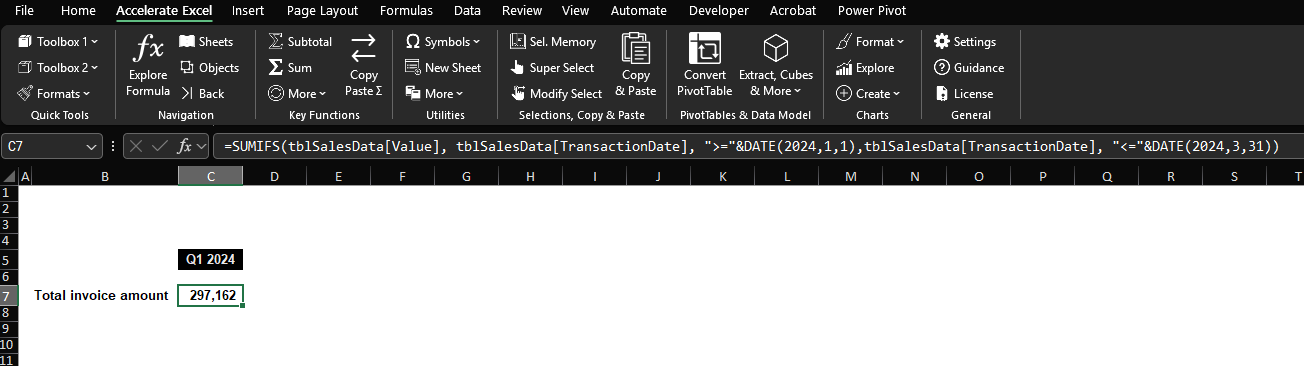
Excel SUMIFS Function: How to aggregate accounting transactions / invoice data between two dates (here Q1 2024).
SUMIFS handles date filters by using comparison operators in the criteria. To sum between two dates, you simply use two criteria on the date column.
=SUMIFS(
        tblSalesData[Value],
        tblSalesData[TransactionDate], ">="&DATE(2024,1,1),
        tblSalesData[TransactionDate], "<="&DATE(2024,3,31)
    )
Here's what each part does:
tblSalesData[Value]: Sum rangeThe column containing the values to be summed.
tblSalesData[TransactionDate]: First criteria rangeThe transaction date column.
">="&DATE(2024,1,1): First criteriaDates on or after January 1, 2024.
tblSalesData[TransactionDate]: Second criteria rangeThe same transaction date column again.
"<="&DATE(2024,3,31): Second criteriaDates on or before March 31, 2024.
SUMIFS Value-Range Formula: Aggregating by Values
Summing by value ranges is also pretty common. Two examples:
Summarize Invoice Data by Size Categories
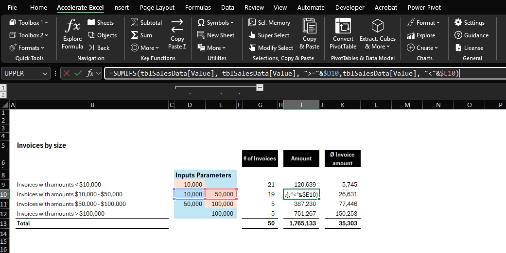
Excel SUMIFS Function: How to categorize accounting transactions / invoice data into value size buckets.
SUMIFS handles value filters by using comparison operators in the criteria. In fact, to sum between two values, you simply use two criteria on the value column:
=SUMIFS(
        tblSalesData[Value],
        tblSalesData[Value], ">="&$D10,
        tblSalesData[Value], "<"&$E10
    )
Here's what each part does:
tblSalesData[Value]: Sum rangeThe column containing the values to be summed.
tblSalesData[Value]: First criteria rangeThe same value column.
">="&$D10: First criteriaValues greater than or equal to the amount in cell D10.
tblSalesData[Value]: Second criteria rangeThe same value column again.
"<"&$E10: Second criteriaValues less than the amount in cell E10.
Note: For counting records instead of summing value , use COUNTIFS with identical criteria but without the sum range:
=COUNTIFS(
        tblSalesData[Value], ">="&$D10,
        tblSalesData[Value], "<"&$E10
    )
Pro tip: You can transform a SUMIFS formula into COUNTIFS by changing the function name and removing the first range argument.
Top Customer Analysis
One of the most common use-cases of SUMIFS in finance are top customer overviews.
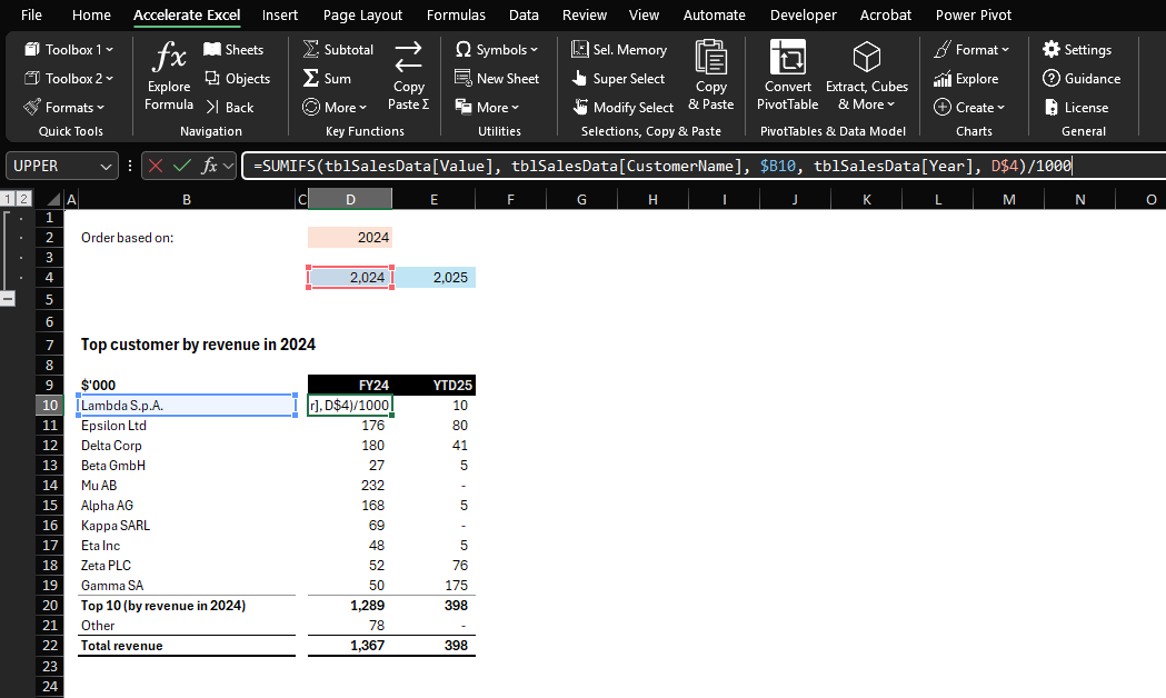
Excel SUMIFS Function: How to create a top customer overview with SUMIFS.
The SUMIFS formula aggregates sales values by customer name and by year:
=SUMIFS(
        tblSalesData[Value],
        tblSalesData[CustomerName], $B10,
        tblSalesData[Year], D$4
    ) / 1000
Here's what each part does:
tblSalesData[Value]: Sum rangeThe column containing the values to be summed.
tblSalesData[CustomerName]: First criteria rangeThe customer name column.
$B10: First criteriaValues where the customer name matches the value in cell B10.
tblSalesData[Year]: Second criteria rangeThe year column.
D$4: Second criteriaValues where the year matches the value in cell D$4.
/1000: After summing the values, the result is divided by 1000 (to convert to thousands for display purposes).
Top Customer Analysis - Excursion (Advanced)
The next few lines cover a more advanced concept. Feel free to skip this section if you’re still getting comfortable with SUMIFS.
The dashboard above incorporates a dynamic dropdown menu (cell D2) that lets you to filter customer sales data by period. When you select a different period, the title (cell B10), subtotal text (cell B20), and top 10 customer rankings automatically update to reflect the new selection.
The core of this functionality is powered by a sophisticated dynamic array formula in cell B10:
=LET(
    year, $D$2,
    customers, UNIQUE(tblSalesData[CustomerName]),
    sales, BYROW(customers, LAMBDA(customerName, SUMIFS(tblSalesData[Value], tblSalesData[CustomerName], customerName, tblSalesData[Year], year))),
    TAKE(SORTBY(customers, sales, -1), 10)
)
This more advanced topic is beyond the scope of this article. However, in simple terms, this formula:
Extracts a unique list of all customers
Calculates total sales for each customer in the selected year
Sorts customers by their sales values (highest to lowest)
Returns only the top 10 performers
Feel free to copy this formula or use our sample workbook to adapt it to your specific needs.
Note: We deliberately separated the complex array formula from the simpler SUMIFS calculations in the dashboard. This modular approach creates a more robust report that won't completely break if one component fails. In a worst-case scenario, you could manually sort and paste the top customer list, and the remaining calculations would still work correctly.
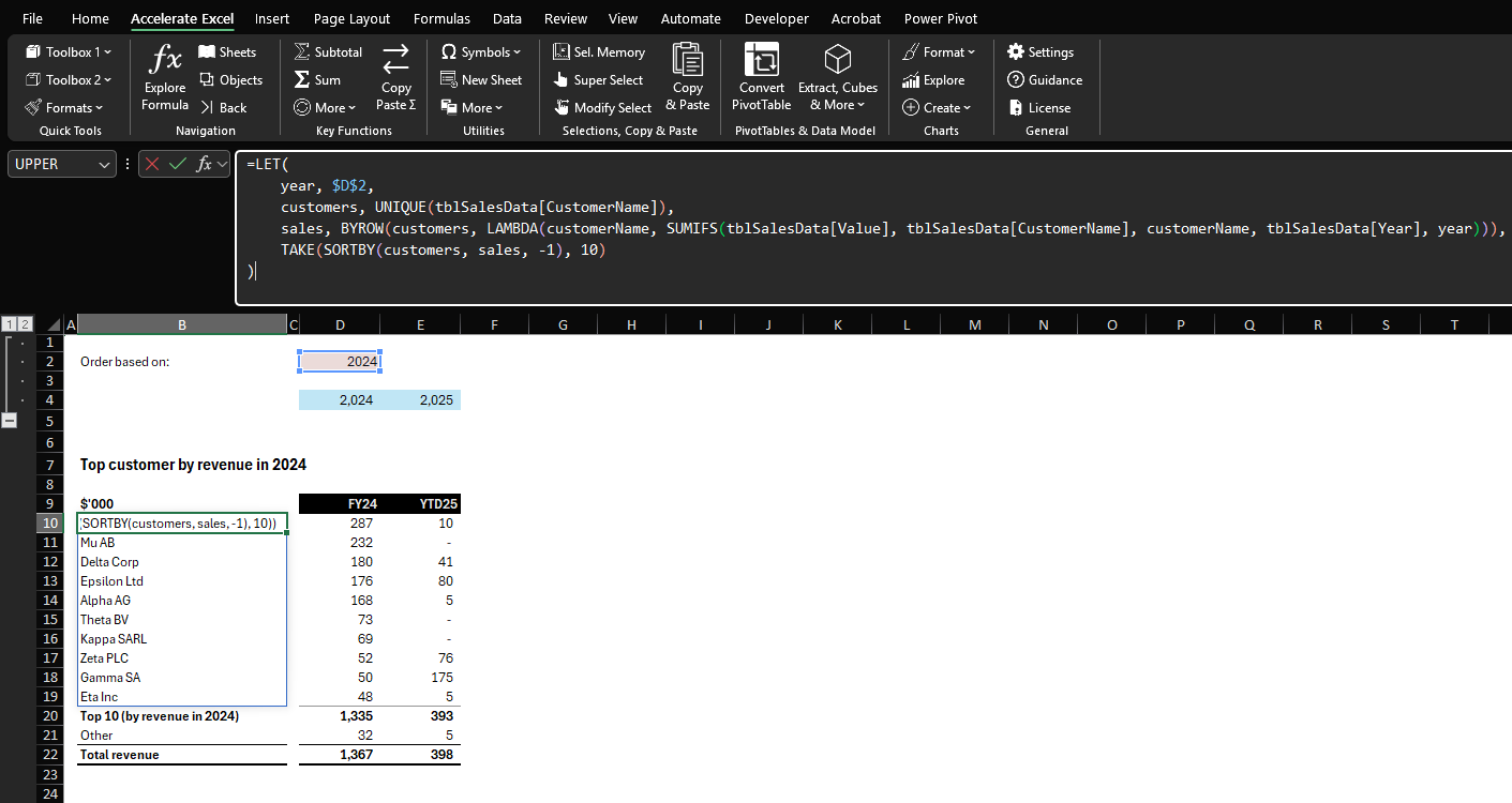
Advanced helper formula to return dynamic and sorted list of top 10 customers.
Best Practices for SUMIFS in Financial Models
Avoid Hardcoding Criteria in Formulas
Wherever possible, link criteria to cells (or use named constants) instead of typing literal values into the formula:
This makes your model interactive – users can change the criteria cell to get a different result.
It prevents mistakes where a hardcoded value becomes outdated or inconsistent.
It’s also easier to spot criteria by looking at the worksheet (no need to inspect the formula bar to know what’s being summed).
Use Tables or Dynamic Ranges
Ensure your SUMIFS ranges expand as data grows. The best way is to convert your data into an Excel Table (Ctrl+T) (or define named ranges that update dynamically):
This way, if new rows are added, your SUMIFS will still capture them.
Using tables also makes formulas easier to read via structured references (e.g.,
Table1[Amount]instead of $C$2:$C$1000). Structured table references improve formula readability and maintainability.
Limit Use of Full Row or Column References
While modern Excel is more optimized for such references, excessive use of full column and/or row references can still slow down your workbooks under certain circumstances. Define specific ranges when possible for better performance.
Ensure Range Alignment
SUMIFS requires that all criteria ranges and the sum range have the same size and orientation (e.g., all three ranges might be A2:A100, B2:B100, and C2:C100).
Always double-check that your ranges line up exactly. If you’re copying formulas across, use absolute references (e.g., $A$2:$A$100) to lock the ranges as needed. A common mistake is a slight misalignment (e.g., one range starting on row 2 and another on row 3), which can lead to wrong results or a zero sum.
Keep Column Headers Consistent
Consistent field names allow you to use the same SUMIFS structure across multiple sheets or datasets without confusion.
For example, if every monthly data sheet has columns labeled Entity, Account, Amount, Year, you can reuse or copy a SUMIFS formula easily. This consistency is crucial in due diligence databooks where multiple files or sheets are involved. It also enables tools (and colleagues) to understand your criteria at a glance, reducing errors.
Avoid Same-Sheet References to Keep Your Formulas Sort-Safe
When you build a SUMIFS on another worksheet, Excel automatically prefixes every in-sheet cell reference with that sheet’s name. If you accept those prefixes—even when the criteria cell lives on the same sheet as the formula—you create a same-sheet reference.
=SUMIFS(
        tblSalesData[Value],
        tblSalesData[CustomerName], 'Example 5_Same Sheet Reference'!$B10,
        tblSalesData[Year], 'Example 5_Same Sheet Reference'!E$4
    ) / 1000
Why it matters
During a sort, Excel treats the prefixed addresses as fixed coordinates. Your data moves, but the formula keeps pointing at the old cells—instantly breaking the logic of your report.
The quick fix
Delete the redundant sheet names (they’re only required when you reference another sheet). The addresses stay relative, so they travel with their rows when you sort.
=SUMIFS(
        tblSalesData[Value],
        tblSalesData[CustomerName], $B10,
        tblSalesData[Year], D$4
    ) / 1000
Tip: After writing your formula, do a quick visual scan for 'current sheet name'!. If you see it, strip it out before you copy, fill, or sort. That one-second check can save hours of troubleshooting later.
Use the Wildcard: *
Wildcards like the asterisk (*) allow for flexible matching of text criteria. The asterisk represents any sequence of characters (including zero characters), making it useful when you need to sum values where text patterns match partially rather than exactly.
Tip: To effectively bypass a condition in your SUMIFS formula without removing it, simply use an asterisk wildcard by itself.
SUMIFS & Accelerate Excel
For professionals who build or audit complex Excel workbook using keyboard shortcuts and other time-saving utilities is a competitive advantage. Accelerate Excel, our specialized Excel add-in, has been made to streamline your Excel workflow. SUMIFS-focused capabilities include:
SUMIFS formula assistant: The tool guides you through building a SUMIFS with just clicks.
This intelligent assistant automatically aligns cell references and builds the formula for you. Even Excel experts appreciate the efficiency. As one user put it: "I never want to write a SUMIFS function manually again."
Convert SUMIFS to direct cell links: Transform complex SUMIFS into transparent calculations with a single click.
This feature lets you replace SUMIFS with a simple SUM that directly references the matching cells. Perfect for auditing, formula validation, and making your data flow / calculations more transparent to others.
The toolkit also improves your SUMIFS-intensive workflow with:
Pivot Table conversion: Instantly transform pivot tables into dynamic formulas (SUMIFS or GETPIVOTDATA).
Dependency visualization: Trace precedents to quickly understand data relationships.
Formatting accelerators: Apply professional styling with specialized shortcuts.
SUMIFS Formula Assistant
Convert SUMIFS to Direct Cell Links
Conclusion
Across financial modeling, M&A analysis, accounting, and strategy consulting, the SUMIFS function transforms raw data into actionable insights through simple yet powerful Excel formulas. SUMIFS is the backbone of most due diligence databooks and many executive dashboards that drive strategic decision-making, making it a must-know for finance professionals.
Having mastered Excel's SUMIFS function, you may be interested in learning more about:
Excel INDEX MATCH formulas. While SUMIFS is the key function for aggregating values, the INDEX MATCH combination excels at lookups based on single or multiple criteria.
Why the SUBTOTAL function is superior to SUM when aggregating values in overviews featuring nested hierarchy levels.
FAQ
How do I use the SUMIFS function in Excel to add numbers that meet several criteria?
Write the formula as =SUMIFS(sum_range, criteria_range1, criteria1, criteria_range2, criteria2…). Excel sums only the rows where all listed criteria are TRUE.
What is the difference between SUMIF and SUMIFS?
SUMIF supports a single criterion, while SUMIFS can evaluate multiple criteria.
How do I build a SUMIFS formula that checks multiple columns at once?
SUMIFS can add only one column per call, so wrap several SUMIFS inside SUM: =SUM( SUMIFS(B:B,$A:$A,"North"), SUMIFS(C:C,$A:$A,"North"), SUMIFS(D:D,$A:$A,"North") ).
Can SUMIFS total values that fall inside a specific date range?
Yes. Pass >= and <= criteria wrapped in quotation marks and concatenated with ampersands, for example: =SUMIFS($D:$D,$B:$B,">="&DATE(2025,1,1),$B:$B,"<="&DATE(2025,1,31)).
Why do my SUMIFS criteria have to be inside quotation marks?
Operators such as ">" or "<>0" are text strings. Double quotation marks tell Excel to treat them as text; without quotes you will see #NAME? or #VALUE! errors.
How can SUMIFS work with wildcards to match partial text?
Use * for any characters and ? for a single character. For example, =SUMIFS(D:D,B:B,"*blue*") totals rows containing the word “blue” anywhere in column B.
Can SUMIFS replace VLOOKUP when I need to return a total instead of a single value?
Often, yes. Where VLOOKUP fetches one cell, SUMIFS can return an aggregate. Example: =SUMIFS(Table[Sales],Table[Product],A2) quickly sums all sales for the product in A2.
When should I switch from SUMIFS to SUMPRODUCT for multi-criteria sums?
Choose SUMPRODUCT if your criteria ranges are different sizes or you need OR logic across columns—two things SUMIFS cannot handle. Otherwise SUMIFS is faster and less prone to accidental array errors.
How do I combine SUMIFS with the IFS function for advanced business rules?
Wrap SUMIFS inside IFS to switch the target column on the fly. Example: =IFS(E2="Q1",SUMIFS(Q1Sales,$A:$A,G2),E2="Q2",SUMIFS(Q2Sales,$A:$A,G2)). The IFS function acts like a routing table for different SUMIFS calls.